Create DAX calculations in semantic models

Mohamad's interest is in Programming (Mobile, Web, Database and Machine Learning). He is studying at the Center For Artificial Intelligence Technology (CAIT), Universiti Kebangsaan Malaysia (UKM).
Adding DAX calculations to Power BI semantic models allows you to define custom logic within your data model, to enable deeper analysis and data-driven business decisions.
Learning objectives
In this module, you learn how to:
Create calculated tables.
Create calculated columns.
Create measures using DAX.
[1] Introduction
When you first create a semantic model by applying Power Query queries, the model consists of tables and columns. At this point, the model probably isn't ready for use. That's because you might need to create or adjust model relationships, create other tables or columns, add hierarchies, or set model properties. You might also identify the need for calculations to summarize the model data, especially when the requirement can't be achieved by summarizing a single column. For example, you might want to calculate year-to-date (YTD) sales revenue, which requires special time filters.
You can use Data Analysis Expressions (DAX) to add three types of calculations to your semantic model to complete your model design:
Calculated tables, which can be useful to create date tables or role-playing dimensions, or to enable what-if analysis.
Calculated columns, which can be added to tables in your model.
Measures, which achieve summarization over model data.
In this module, you learn why and how to create each of these calculation types.
[2] Create calculated tables
A calculated table is created with a DAX formula that returns a table object, allowing you to duplicate or transform existing model data to produce a new table.
Duplicate a table
A common design challenge in data modeling is handling multiple relationships between tables. For example, the Sales table might have three relationships to the Date table, as shown in the following diagram:

The Sales table stores sales data by order date, ship date, and due date, resulting in three relationships to the Date table. However, only one relationship can be active at a time, as indicated by a solid line in the diagram. The other relationships are inactive and shown as dashed lines.
In our example, the active relationship filters the OrderDateKey column in the Sales table, so filters applied to the Date table affect sales by order date only.
To enable filtering sales by ship date, a new table can be created by duplicating the Date table with the following formula:
DAXCopy
Ship Date = 'Date'
This formula creates a new table named Ship Date with the same columns and rows as the original Date table. When the Date table is refreshed, the Ship Date table is also recalculated to remain synchronized. Now you can create an active relationship between Ship Date and Sales tables to allow filtering by ship dates too.
Configure duplicate tables
When you create a calculated table, you need to apply any custom configurations to the new duplicate table you want carried over. For instance, it's a good idea to rename columns so that they better describe their purpose.
In our example, the Fiscal Year column in the Ship Date table can be renamed as Ship Fiscal Year. The Ship Full Date column should be sorted by the Ship Date column and the MonthKey column can be hidden to improve sorting and reporting.
Calculated tables are useful to work in scenarios when multiple relationships between two tables exist, as previously described. However, calculated tables increase the model's storage size and can prolong data refresh times, especially when they depend on other tables.
Note
While duplicate tables solve this challenge, there are other more performant solutions. We cover this concept again when discussing measures later in this module.
Create a date table
A good use case for calculated tables is to add a date table to your model. Date tables are required to apply special time filters known as time intelligence.
You can create a calculated date table using the CALENDARAUTO function. The CALENDARAUTO function scans all date and date/time columns in the model to determine the earliest and latest dates, then generates a complete set of dates that span all years in the data. The argument specifies the last month of the financial year; for example, passing 6 sets June as the year end.
DAXCopy
Due Date = CALENDARAUTO(6)
The resulting Due Date table contains a single column of dates. The following image shows the Due Date table in data view, with dates sorted from earliest to latest:

Tip
The CALENDAR function can also be used to create a date table by specifying a start and end date, either as static values or as expressions based on model data.
If the earliest date in the model is October 15, 2021, and the latest is June 15, 2022, the function returns dates from July 1, 2021, to June 30, 2022. This ensures the table includes complete years, which is required for marking a date table.
Mark as a date table
Once you create a date table, you need to Mark it as a date table in Power BI Desktop. This setting allows you to use time intelligence functions in DAX calculations. When you specify your own date table, Power BI Desktop performs the following validations of that column and its data, to ensure that the data contains:
Unique values.
No null values.
Contiguous date values (from beginning to end).
Same timestamp across each value for Date/Time data types.
This setting applies to any date tables, either imported or created in Power Query or calculated tables.
Note
You must either use a custom date table or use the built-in auto/date time feature in Power BI to use time intelligence. The auto/date time feature has limited values and can't be customized, which is one reason to consider using a custom date table.
[3] Create calculated columns
Occasionally, you need more columns than exist in your data. Ideally, you add these columns directly to the data source, which supports easier maintenance and allows the column logic to be reused in other models or reports. However, if you need to add the column once connected to the data in Power BI, you can either create a custom column in Power Query Editor or add a calculated column to the semantic model. No matter how you add the column, the result is the same from a report user's perspective.
In general, custom columns in Power Query are preferred because they're loaded into the model in a more compact and optimal way. Calculated columns are recommended only when adding columns to a calculated table or when the formula:
Depends on summarized model data.
Requires specialized modeling functions available only in DAX, such as
RELATED,RELATEDTABLE, or functions for parent-child hierarchies.
Create calculated columns
A DAX formula can be used to add a calculated column to any table in the model. The formula must return a single value (scalar) for each row.
Calculated columns in import models increase storage size and can prolong data refresh times, especially when they depend on other tables that are refreshed. Therefore, be cautious when using too many calculated columns and consider if a measure can be used instead.
In the following examples, several calculated columns are created to support fiscal analysis to demonstrate the versatility of calculated columns.
Fiscal Year
This column determines the fiscal year for each date. The fiscal year starts in July, so dates from July to December are assigned to the next calendar year. The formula concatenates "FY" with the year, incrementing the year by one for dates in the second half of the year.
DAXCopy
Due Fiscal Year =
"FY"
    & YEAR('Due Date'[Due Date])
        + IF(
            MONTH('Due Date'[Due Date]) > 6,
            1
        )
The following steps describe how Microsoft Power BI evaluates the calculated column formula:
The addition operator (+) is evaluated before the text concatenation operator (&).
The
YEARfunction returns the whole number value of the due date year.The
IFfunction returns the value when the due date month number is 7-12 (July to December); otherwise, it returns BLANK. (For example, because the Adventure Works financial year is July-June, the last six months of the calendar year will use the next calendar year as their financial year.)The year value is added to the value that is returned by the
IFfunction, which is the value one or BLANK. If the value is BLANK, it's implicitly converted to zero (0) to allow the addition to produce the fiscal year value.The literal text value
"FY"concatenated with the fiscal year value, which is implicitly converted to text.
Fiscal Quarter
This column assigns a fiscal quarter to each date, based on the fiscal year structure where Quarter 1 is July–September. The formula appends Q and the quarter number to the fiscal year label.
DAXCopy
Due Fiscal Quarter =
'Due Date'[Due Fiscal Year] & " Q"
    & IF(
        MONTH('Due Date'[Due Date]) <= 3,
        3,
        IF(
            MONTH('Due Date'[Due Date]) <= 6,
            4,
            IF(
                MONTH('Due Date'[Due Date]) <= 9,
                1,
                2
            )
        )
    )
Month Key
The MonthKey formula multiplies the due date year by the value 100 and then adds the month number of the due date. It produces a numeric value that can be used to sort the Due Month text values in chronological order.
DAXCopy
MonthKey =
(YEAR('Due Date'[Due Date]) * 100) + MONTH('Due Date'[Due Date])
Full Date Label
The FORMAT function converts the Due Date column value to text by using a format string. In this case, the format string produces a label that describes the year, abbreviated month name, and day:
DAXCopy
Due Full Date =
FORMAT('Due Date'[Due Date], "yyyy mmm, dd")
Note
Many user-defined date/time formats exist. For more information, see Custom date and time formats for the FORMAT function.
After these additions, the Due Date table contains six columns: the original date column and five calculated columns. These columns support both time intelligence functions and readability for report consumers.

Understand row context
Power BI evaluates a calculated column’s formula for each row in the table, which is called row context. Row context just means “the current row.” For example, here’s the Due Fiscal Year calculated column:
DAXCopy
Due Fiscal Year =
"FY"
    & YEAR('Due Date'[Due Date])
        + IF(
            MONTH('Due Date'[Due Date]) <= 6,
            1
        )
When Power BI runs this formula, 'Due Date'[Due Date] gives the value from the current row. If you’ve used Excel tables, this idea might feel familiar.
Row context only applies to the current table. If you need values from another table, you have two main options:
If a relationship exists between the two tables, use the
RELATEDorRELATEDTABLEfunction.RELATEDgets a value from the one-side of a relationship.RELATEDTABLEgets a table of values from the many-side.If there's no relationship, use the
LOOKUPVALUEfunction.
Try to use RELATED when you can. It usually works faster than LOOKUPVALUE because of how Power BI stores and indexes data.
Here’s an example. This formula adds a Discount Amount column to the Sales table:
DAXCopy
Discount Amount =
(
    Sales[Order Quantity]
        * RELATED('Product'[List Price])
) - Sales[Sales Amount]
Power BI calculates this formula for each row in the Sales table. It gets Order Quantity and Sales Amount from the current row. To get List Price from the Product table, it uses the RELATED function to find the right value for each sale.
Row context always applies when Power BI evaluates calculated column formulas. It also comes into play with iterator functions, which let you create more advanced summaries. You learn about iterator functions later in this module.
[4] Understand implicit measures
Measures in Power BI models are either implicit or explicit. Implicit measures are automatic behaviors that let visuals summarize column data. Explicit measures, often called measures, are calculations you add to your model. This section explains how implicit measures work and how you can use them.
Identify implicit measures
As a data modeler, you control how a column summarizes by setting the Summarization property. You can choose Don't summarize or select a specific aggregation function. If you set a column to Don't summarize, the sigma symbol disappears in the Data pane.
In the Data pane, a column with the sigma symbol (∑) shows two facts:
The column is numeric.
Values are summarized when used in a visual that supports summarization.
The following image shows the Sales table with implicit measures, a calculated column, and one column that can't be summarized.

Notice in the example with the Sales table, if you add the Sales Amount field from the Sales table to a matrix visual that groups by fiscal year and month, Power BI summarizes the values implicitly. The Sum aggregation function is selected by default.

If you add the Unit Price field to the matrix visual, Power BI uses Average as the default summarization, because summing unit prices doesn’t make sense since they’re rates, not totals.

The default summarization is now set to Average (the modeler knows that it's inappropriate to sum unit price values together because they're rates, which are non-additive).
Implicit measures allow the report author to start with a default summarization technique and lets them modify it to suit their visual requirements. Numeric columns support the widest range of aggregation functions to choose from, including:
Sum
Average
Minimum
Maximum
Count (Distinct)
Count
Standard deviation
Variance
Median
Summarize non-numeric columns
Non-numeric columns like text, dates, and boolean (true/false) values can also be summarized in your visuals. While the sigma symbol (∑) only appears next to numeric fields in the Data pane, these columns are still being aggregated.
Text columns: First, Last, Count, Count (Distinct)
Date columns: Earliest, Latest, Count, Count
This flexibility is useful when you want to answer questions such as:
"How many unique products are there?" (Count distinct on a text column)
"What was the earliest order date?" (Earliest on a date column)
"How many orders were marked as complete?" (Count on a boolean column)
You can choose the aggregation option that best fits your analysis when you add a non-numeric field to your visual.
Considerations for implicit measures
Implicit measures are easy to use and flexible. They let report authors start with a default summarization and change it to fit their needs. Implicit measures let report authors quickly visualize data without needing to write calculations. As a data modeler, you spend less time creating explicit measures.
However, even if you set a default summarization, report authors can change it to something that might not make sense. For example, they could set Unit Price to Sum, which produces misleading results, as shown in the following image. The Unit Price values are large because they're the sum of unit prices instead of the static unit price per product.

The biggest limitation is that implicit measures only work for simple scenarios. They can summarize column values using a single aggregation function, but they can’t handle more complex calculations. For example, if you need to calculate the ratio of each month’s sales amount over the yearly sales amount, you must create an explicit measure with a DAX formula.
[5] Create explicit measures
You can add a measure to any table in your model by writing a DAX formula. A measure formula must return a single value. This section explains how to create explicit measures.
Measures don’t store values in the model. Instead, Power BI calculates them at query time to summarize model data. Measures can’t reference a table or column directly, so you must use a function to summarize the data.
Simple measures
A simple measure aggregates the values of a single column, just like an implicit measure.
For example, you can add a measure to the Sales table. In the Data pane, select the Sales table. On the Table Tools ribbon, select New measure.

The following formula creates a measure called Revenue. This measure uses the SUM function to total the values in the Sales Amount column. If you add this measure to a table alongside the Sales Amount implicit measure, the results are the same.
DAXCopy
Revenue =
SUM(Sales[Sales Amount])
Tip
Adding measures and hiding columns helps report authors use the explicit measures instead.
In the Measure tools contextual ribbon, you can format the measure, set data type, and change the home table. The home table refers to where the measure shows when looking at the data pane.

Tip
It's a good practice to set the formatting options right after you create a measure. This ensures your values look consistent in all report visuals.
Consider you might need a measure to calculate Profit as shown in the following code:
DAXCopy
Profit =
SUM(Sales[Profit Amount])
In this example, the Profit Amount column is a calculated column. This approach isn’t optimal because you don’t need that column. In the next section, you see how to create a measure that calculates profit directly, which reduces model size and improves refresh times.
The following code creates two different measures to return Order Line Count and Order Count. The COUNT function counts non-BLANK values in a column. The DISTINCTCOUNT function counts unique values. Since an order can have multiple order lines, the Sales Order column has duplicates. Using DISTINCTCOUNT gives you the correct order count.
DAXCopy
Order Line Count =
COUNT(Sales[SalesOrderLineKey])

Order Count =
DISTINCTCOUNT('Sales Order'[Sales Order])
You can also write the Order Line Count measure using COUNTROWS, which counts the number of rows in a table:
DAXCopy
Order Line Count =
COUNTROWS(Sales)
All the measures referenced are considered simple measures because they aggregate a single column or single table.
Create compound measures
A compound measure references one or more other measures. For example, you can redefine the Profit measure by referencing other measures. This measure can be used instead of the calculated column previously referenced.
DAXCopy
Profit =
[Revenue] - [Cost]
This change to the model presents an important lesson: By removing the calculated column, you optimize the semantic model because it results in a decreased semantic model size and shorter data refresh times. The Profit Amount calculated column wasn't required after all because the Profit measure can directly produce the required result by using existing measures.
Note
Sometimes, it makes sense to define measures that depend on other measures. Always test changes carefully, because updates can affect all dependent measures.
Use Quick measures
Quick measures let you perform common calculations without writing DAX yourself. Power BI generates the DAX expression for you, which helps you learn and build your DAX skills.
For example, you can use a Quick measure to create a Profit Margin measure through the following steps:
Select Quick measure in the Table tools ribbon.
Choose Mathematical operations > Division.
Add the
Profitmeasure into Numerator andRevenueinto Denominator.

The new measure appears in the Data pane, and you can review its DAX formula:
DAXCopy
Profit Margin =
DIVIDE([Profit], [Revenue])
Compare calculated columns and measures
Many DAX beginners find calculated columns and measures confusing at first. Both are created in the semantic model using DAX formulas, however, calculated columns and measures behave differently.
Expand table
| Calculated columns | Measures | |
| Purpose | Adds a new column to a table | Defines how to summarize model data |
| Evaluation | Evaluated using row context at data refresh time | Evaluated using filter context at query time |
| Storage | Stores a value for each row in the table (Import mode) | Never stores values in the model |
| Use in visuals | Can filter, group, or summarize data (as implicit measures) | Designed specifically to summarize data |
| Performance impact | Can increase memory usage and model size | More efficient; better performance in large models |
| Ideal for | New fields for slicing or relationships | Dynamic calculations based on filters |
Recognizing these differences helps you choose the right approach for your modeling and reporting needs.
[6] Use iterator functions
Iterator functions evaluate an expression for each row in a table. They give you flexibility and control over how your model summarizes data.
Single-column summarization functions, such as SUM, COUNT, MIN, and MAX, have equivalent iterator functions with an "X" suffix, like SUMX, COUNTX, MINX, and MAXX. Specialized iterator functions also exist for filtering, ranking, and semi-additive calculations over time.
Every iterator function requires a table and an expression. The table can be a model table or any expression that returns a table. The expression must return a single value for each row.
Single-column summarization functions, like SUM, act as shorthand. Power BI internally converts SUM to SUMX. For example, both of the following measures return the same result and have the same performance:
DAXCopy
Revenue = SUM(Sales[Sales Amount])
DAXCopy
Revenue =
SUMX(
    Sales,
    Sales[Sales Amount]
)
Iterator functions evaluate the expression for each row in a table, using row context—meaning they process one row at a time to compute the final result. Then the table is evaluated in filter context. For example, if a report visual filters by fiscal year FY2020, the Sales table contains only sales rows from that year.
Important
Using iterator functions with large tables and complex expressions can slow performance. Functions like SEARCH and LOOKUPVALUE can be expensive. When possible, use RELATED for better performance.
Iterator functions for complex summarization
Iterator functions let you aggregate more than a single column. For example, a revenue measure can multiply order quantity, unit price, and a discount factor for each row, then sum the results.
DAXCopy
Revenue =
SUMX(
    Sales,
    Sales[Order Quantity] * Sales[Unit Price] * (1 - Sales[Unit Price Discount Pct])
)
Iterator functions can also reference related tables. The discount measure can use the RELATED function to access the list price from the product table:
DAXCopy
Discount =
SUMX(
    Sales,
    Sales[Order Quantity]
    * (
        RELATED('Product'[List Price]) - Sales[Unit Price]
    )
)
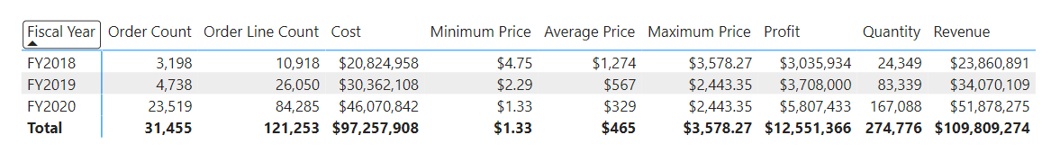
The following image shows a table visual with the Month, Revenue, and Discount columns. Revenue and Discount are the measures previously created.

Iterator functions for higher grain summarization
Iterator functions can also summarize data at different levels of detail (grain). For example, you might want to calculate an average at the line item level or at the sales order level.
In this example, the Sales table contains one row for each line item in a sales order. Each row includes details such as the sales order number, product, quantity sold, unit price, and discount. Multiple rows can have the same sales order number, representing different items within the same order.
To calculate the average revenue per order line (line item), you can use the AVERAGEX function to iterate over each row in the Sales table. The formula calculates revenue for each line item, then averages the result across all line items in the current filter context:
DAXCopy
Revenue Avg Order Line =
AVERAGEX(
    Sales,
    Sales[Order Quantity] * Sales[Unit Price] * (1 - Sales[Unit Price Discount Pct])
)

If you want to calculate the average revenue per sales order (rather than per line item), you can use the VALUES function to get a list of unique sales order numbers first. Then, AVERAGEX iterates over each sales order and averages the total revenue for each order:
DAXCopy
Revenue Avg Order =
AVERAGEX(
    VALUES('Sales Order'[Sales Order]),
    [Revenue]
)
The VALUES function returns the unique sales orders based on the current filter context, so AVERAGEX iterates over each sales order for each month.

Ranking with iterator functions
The RANKX function calculates ranks by iterating over a table and evaluating an expression for each row.
Order direction can be ascending or descending. Ranking revenue usually uses descending order, so the highest value ranks first. Ranking something like complaints might use ascending order, so the lowest value ranks first. By default, RANKX uses descending order and skips ranks for ties.
For example, a product quantity rank measure can use RANKX and the ALL function to rank products by quantity:
DAXCopy
Product Quantity Rank =
RANKX(
    ALL('Product'[Product]),
    [Quantity]
)
The ALL function removes filters, so RANKX ranks all products. In the following image, two products tie for tenth place, so the next product is ranked twelfth and rank 11 is skipped.
![]()
You can also use dense ranking, which assigns the next rank after a tie without skipping numbers. To use dense ranking, the measure can include the DENSE argument:
DAXCopy
Product Quantity Rank =
RANKX(
    ALL('Product'[Product]),
    [Quantity],
    ,
    ,
    DENSE
)
Now, after two products tie for tenth place, the next product is ranked eleventh and numbering continues sequentially without skipping rank 11.
![]()
In this visual, the total row for the Product Quantity Rank measure shows one, because the total for all products is also ranked and there's only one value.
![]()
To avoid ranking the total, the measure can use the HASONEVALUE function to return BLANK unless a single product is filtered:
DAXCopy
Product Quantity Rank =
IF(
    HASONEVALUE('Product'[Product]),
    RANKX(
        ALL('Product'[Product]),
        [Quantity],
        ,
        ,
        DENSE
    )
)
Now, the total for Product Quantity Rank is blank.
![]()
The HASONEVALUE function checks if the product column has a single value in filter context. This is true for each product group, but not for the total, which represents all products.
Iterator functions provide powerful ways to summarize, aggregate, and rank data in Power BI models. They support complex calculations and let you control the level of detail in your reports.
[7] Exercise - Create DAX calculations
Completed100 XP
- 45 minutes
This unit includes a lab to complete.
Use the free resources provided in the lab to complete the exercises in this unit. You will not be charged for the lab environment; however, you may need to bring your own subscription depending on the lab.
Microsoft provides this lab experience and related content for educational purposes. All presented information is owned by Microsoft and intended solely for learning about the covered products and services in this Microsoft Learn module.
In this exercise, you learn how to use DAX to:
Create calculated tables.
Create calculated columns.
Create measures.
This lab takes approximately 45 minutes to complete.
Note
A virtual machine containing the client tools you need is provided, along with the exercise instructions. Use the "Launch lab" button to launch the virtual machine.
A limited number of concurrent sessions are available. If the hosted environment is unavailable, please try again later.
Alternatively, you can open the instructions in a separate window.
Access your environment
Before you start this lab (unless you are continuing from a previous lab), select Launch lab above.
You are automatically logged in to your lab environment as data-ai\student.
You can now begin your work on this lab.
Tip
To dock the lab environment so that it fills the window, select the PC icon at the top and then select Fit Window to Machine.

[8] Check your knowledge
[1] Which statement about calculated tables is true?
a. Calculated tables increase the size of the semantic model.
b. Calculated tables are evaluated by using row context.
c. Calculated tables are created in Power Query.
d. Calculated tables can't include calculated columns.
[2] Which statement about calculated columns is true?
a. Calculated columns are created in the Power Query Editor window.
b. Calculated column formulas are evaluated by using row context.
c. Calculated column formulas can only reference columns from within their table.
d. Calculated columns can't be related to noncalculated columns.
[3] Which statement about measures is correct?
a. Measures store values in the semantic model.
b. Measures must be added to the semantic model to achieve summarization.
c. Measures can reference columns directly.
d. Measures can reference other measures directly.
[9] Summary
This module covered using DAX calculations to extend your semantic model. You learned the differences between calculated columns and measures, including when and how Power BI evaluates them and how they store data. Explicit measures are important because they allow you to create complex DAX formulas to achieve the precise calculations that your report visuals need.
You also learned how calculated columns are evaluated within row context, and iterator functions are available in measures for advanced row-by-row calculations.
Understanding how to create and use DAX calculations is fundamental for building effective, flexible, and maintainable semantic models in Power BI. These concepts help you design reports that deliver accurate insights and support a wide range of analytical requirements.
For more information, see Introduction to DAX in Power BI.
Source:
https://learn.microsoft.com/en-us/training/modules/dax-power-bi-create-calculations/